Essential Spreadsheet Formulas Every User Should Know

Did you know the average office worker spends over 400 hours a year on repetitive data tasks? I have discovered that mastering a few key digital shortcuts can instantly reclaim that lost time. By learning these spreadsheet formulas, you can stop manual entry and let your software handle the heavy lifting.

View original

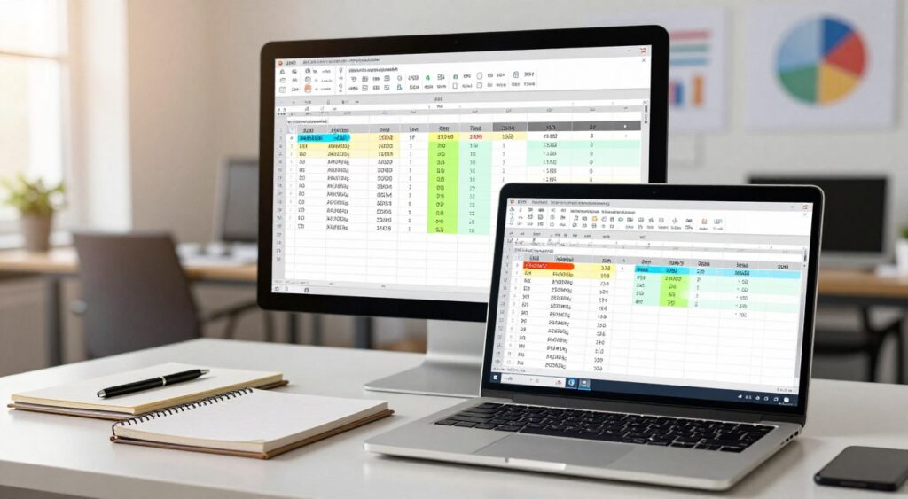
spreadsheet formulas

I aim to offer a clear formula guide that simplifies complex calculations. Whether you’re using Excel or Google Sheets, understanding references, conditions, and lookups will transform your work. I’ll share practical formula examples to boost your confidence in organizing data.

You’ll also find valuable formula tips for handling dates and fixing common errors. This foundation ensures your work remains accurate and professional every day.

Key Takeaways

• Save hundreds of hours by automating repetitive data entry tasks.
• Master essential functions for both Excel and Google Sheets platforms.
• Improve data accuracy through better error handling and logic.
• Learn to organize information efficiently using advanced lookup tools.
• Build a reliable foundation for all your future data projects.

Build a Reliable Formula Workflow in Excel and Google Sheets

Data analysts who excel follow a consistent formula-writing process. This approach minimizes errors and boosts productivity. Whether using Excel formulas or Google Sheets formulas, a structured method keeps work professional and auditable.

 Identify the calculation before choosing a function

Before starting, define your goal clearly. I suggest outlining the logic on paper or in a note. This helps avoid using overly complex spreadsheet formulas when simpler ones will do.

Start every formula with an equals sign.

Every calculation must begin with an equals sign (=). This tells the program it’s a command, not text. Forgetting this can confuse the application, making data analysis harder.

Use cell references instead of hard-coded values.s

Using cell references is crucial. It makes your Excel formulas update automatically with data changes. This flexibility is essential for scalable spreadsheets.

Check formula results for accuracy and consistency

Always double-check your work. I verify my outputs against a manual sample to ensure accuracy. Consistency is vital, whether for team or client use.

Understand Cell References and Formula Shortcuts

Mastering cell references is key to creating robust, error-free models in your spreadsheet. When crafting Excel formulas, how you reference data affects their behavior when moved or copied. This is crucial for maintaining accuracy in large datasets.

Grasping these concepts is a valuable formula tip for ensuring data integrity across vast datasets.

Use relative references for formulas that need to move

Most spreadsheets default to relative references. Copying a formula adjusts cell addresses based on position changes. This is incredibly efficient for tasks requiring the same operation on different rows or columns.

For instance, adding two cells in row one and copying the formula down adjusts references to row two. This flexibility is essential for repetitive tasks.

Lock rows and columns with absolute references.

At times, a specific cell must remain constant when copying formulas. Using the dollar sign ($) symbol creates an absolute reference. This is vital for operations involving a single tax rate or conversion factor stored in one cell.

Adding a $ before the column letter and row number locks that cell. This is crucial for operations like multiplying a range by a constant value.

Combine relative and absolute references with mixed references

Mixed references allow locking either the row or column while keeping the other flexible. This is useful for complex tables needing simultaneous calculations across dimensions.

Locking a column ensures formulas pull from the correct category as you drag them across rows. This is a critical formula tip for advanced data analysis.

Copy formulas safely with fill handles and keyboard shortcuts

The fill handle, a small square at a cell’s bottom-right corner, is perfect for propagating formulas. Dragging this handle is the quickest way to apply your logic across a range.

For those preferring keyboard shortcuts, using formula shortcuts like Ctrl+D to fill down or Ctrl+R to fill right saves time. These methods ensure accurate reference updates without manual re-entry.

Recognize when pasted formulas need reference adjustments

When copying and pasting Excel formulas between sheets or workbooks, references might not match the intended data. Always verify your ranges post-pasting to maintain logical consistency.

Unexpected results? Use the F2 key to inspect cell references visually. This habit prevents errors and keeps your Excel formulas reliable as your project expands.

Calculate Totals and Basic Statistics with Core Spreadsheet Formulas

Transforming raw numbers into meaningful insights is possible with a few key spreadsheet formulas. These tools enable quick summarization of large datasets, laying a solid foundation for reports. Mastering these calculation functions saves time and minimizes the chance of manual errors.

Use SUM to add ranges, columns, and selected cells

The SUM function is a staple for data aggregation. It effortlessly adds up entire columns or specific cell ranges. Simply enter =SUM(range) to instantly total your selected values.

Use AVERAGE to calculate a meaningful mean.

For understanding a dataset’s central tendency, the AVERAGE function is indispensable. It calculates the arithmetic mean by summing all numbers and dividing by their count. This is invaluable for analyzing performance or sales trends.

Use MIN and MAX to find the smallest and largest values

Spotting data extremes is crucial for identifying outliers or peak performance periods. MIN returns the lowest value, while MAX finds the highest. These calculation functions are essential for setting data analysis boundaries.

Use COUNT and COUNTA to measure numeric and nonblank entries

Tracking record counts is vital for data integrity. COUNT tallies numeric cells, whereas COUNTA counts all non-empty cells. Here’s how they differ:

• COUNT: Ideal for tracking numeric data like prices or dates.
• COUNTA: Useful for counting text, labels, or mixed data types.

Choose COUNTBLANK when missing data matters.

At times, the most critical information is what’s missing. The COUNTBLANK function identifies empty cells, ensuring data completeness before report finalization.

Apply Conditional Calculations with IF and Related Functions

Effective spreadsheets make decisions automatically based on their values. By using calculation functions, you can turn static data into a dynamic tool. This allows your workbook to perform different actions based on conditions.

Write a basic IF formula with a true and false result

The IF function is the foundation of logical testing. It checks a condition and returns one value if true, another if false. For example, a formula like =IF(A1>100, “High”, “Low”) categorizes sales figures instantly.

Build multiple outcomes with nested IF statements.

At times, a simple true or false result is insufficient. Nesting multiple IF statements creates a chain of logic. While powerful, it can become complex with more than three or four conditions.

Use IFS for clearer multi-condition logic.

IFS is recommended for avoiding clutter in formulas. It tests multiple conditions in a single line of code. It returns the value associated with the first true condition.

Combine IF with AND and OR to test several requirements

Nesting AND or OR functions within IF statements expands your logic. The AND function requires all conditions to be met. The OR function triggers a result if at least one condition is true. These calculation functions are crucial for complex reporting.

Use NOT when a condition must be reversed.

Sometimes, you need to act only when a condition is not met. The NOT function reverses the logical value of an argument. This is useful for flagging items outside a desired range.

Return blank cells instead of distracting zero values

Unwanted zeros can be a frustration in spreadsheets. You can solve this by returning an empty string instead of zero. Using “” at the end of your IF statement keeps reports clean and professional.

• IF: The primary tool for logical branching.
• IFS: Best for handling multiple conditions without nesting.
• AND/OR: Used to combine multiple logical tests.
• Empty String: A simple trick to hide zero values in your output.

Summarize Data with COUNTIF, SUMIF, and AVERAGEIF

The most powerful insights in a spreadsheet often come from conditional summary functions. These tools help extract specific answers from large datasets without manual filtering. By using these formula examples, you can automate your reporting and save a lot of time.

Count matching records with COUNTIF.

The COUNTIF function is ideal for counting items that meet a single requirement. For example, I use it to count sales orders in a specific region. It scans a range and returns the total count of cells that match my criteria.

Add values that meet a condition with SUMIF.

When I need to calculate a total based on a category, I use SUMIF. This function adds up corresponding values in another range if they meet my condition. These formula examples are crucial for tracking monthly budgets or sales performance by department.

Average only qualifying values with AVERAGEIF

Calculating a mean can be misleading if irrelevant data points are included. The AVERAGEIF function isolates specific subsets, like the average price of products in a certain category. It ensures my final metrics are highly accurate and relevant to my business goals.

Use COUNTIFS, SUMIFS, and AVERAGEIFS for multiple criteria

When a single condition is not enough, the plural versions of these functions are necessary. These advanced tools allow me to layer multiple requirements, such as filtering by both date and region. They are essential for complex, professional-grade dashboards.

Set criteria for text, numbers, dates, and partial matches

You can define criteria using exact text, numeric thresholds, or date ranges. I often use wildcards like the asterisk (*) for partial matches. This flexibility makes your analysis robust and adaptable.

“Data is the new oil, but it is useless unless you have the right tools to refine it into actionable insights.”

— Anonymous

Keep criteria flexible by referencing cells

Hard-coding values into a formula is rarely a good practice. Instead, I prefer to reference a specific cell that contains the criteria. This allows me to update my report instantly by changing a single input cell, rather than editing every formula individually.

By mastering these formula examples, you will transform how you interact with your data. Whether you are counting, summing, or averaging, these functions provide the precision needed for effective decision-making in any professional environment.

Clean and Combine Text with Essential Text Formulas

Raw data often needs a thorough cleanup before it’s useful. Whether it’s importing customer lists or merging reports, text manipulation is crucial. These tools help standardize entries and prepare data for deeper analysis.

Join names and labels with CONCAT and TEXTJOIN.

When merging data, like combining first and last names, I turn to concatenation. CONCAT works well for simple merges. But TEXTJOIN excels by allowing specific delimiters, like commas or spaces, between values.

Extract characters with LEFT, RIGHT, and MID.

At times, I only need a part of a cell’s content. LEFT and RIGHT functions extract characters from the start or end. For more precise needs, MID isolates text from any position.

Measure text length with LEN.

LEN is my top choice for data quality checks. It counts characters in a cell, helping spot short entries or errors. This simple yet highly effective method ensures consistency in large datasets.

Remove unwanted spaces with TRIM.

Imported data often has extra spaces, causing errors and formatting issues. TRIM removes leading, trailing, and double spaces. This formula guide technique keeps spreadsheets clean, preventing calculation mistakes.

Change capitalization with UPPER, LOWER, and PROPER.

Standardizing report appearance is key for professionalism. I use UPPER for all caps, LOWER for lowercase, and PROPER for proper case. These functions ensure uniform, polished labels.

Use TEXT to display numbers and dates in readable formats

The TEXT function is special because it converts numbers and dates into text strings. I use it to format dates as “MM/DD/YYYY” or add currency symbols. This makes my output easy to read for all.

Work with Dates, Times, and Scheduling Calculations

Mastering date and time logic is key to creating dynamic spreadsheets. By using specific calculation functions, you can automate project timelines. This ensures your data stays current without manual updates.

Insert the current date with TODAY.

The TODAY function is a simple yet powerful tool. It returns the current date. Being a volatile function, it updates automatically every time you open your file or perform a new calculation.

Insert the current date and time with NOW.

For tracking precise moments, the NOW function is ideal. It captures both the current date and exact time. This is essential for logging entries or tracking task durations.

Calculate elapsed time by subtracting dates.

Subtracting one date from another easily determines the number of days between events. Spreadsheets treat dates as serial numbers, making this math straightforward and reliable for project tracking.

Extract date components with DAY, MONTH, and YEAR

Sometimes, isolating specific date parts is necessary for reporting. The DAY, MONTH, and YEAR functions allow you to extract these values into separate columns. This makes grouping data by fiscal periods or seasonal trends easier.

Calculate working days with NETWORKDAYS.

When planning project schedules, excluding weekends is crucial for an accurate count of business days. The NETWORKDAYS function simplifies this by calculating the total number of workdays between two dates.

Account for holidays and nonstandard workweeks

Professional projects often require more than a standard Monday-through-Friday schedule. Including a list of holidays in your Google Sheets formulas ensures your timeline accounts for company closures or regional bank holidays.

• Create a separate range for your holiday dates.
• Reference this range within the NETWORKDAYS function.
• Adjust your logic if your organization operates on a nonstandard workweek.

Move dates forward or backward with EDATE and EOMONTH

Managing recurring deadlines is easier with EDATE and EOMONTH. EDATE shifts a date by a specific number of months. EOMONTH finds the final day of a month, which is incredibly useful for monthly financial reporting and subscription billing cycles.

Find, Match, and Retrieve Data from Tables

Locating specific values in a large table is a common challenge for spreadsheet users. These tools help automate workflows and ensure data accuracy without manual searches. By mastering these Excel formulas, you can easily link different datasets.

Use VLOOKUP for straightforward vertical searches.

The VLOOKUP function is ideal for vertical searches in the first column of a range. It fetches data from the same row in a corresponding column. It’s most beneficial for data organized in a simple vertical list.

Use HLOOKUP when lookup values run across rows.

For horizontally oriented data, HLOOKUP is the go-to alternative. It scans the top row of a table and returns a value from a specified row below. These formula examples show how to adjust your approach based on your table’s layout.

Build flexible searches with INDEX and MATCH.

Many experts prefer INDEX and MATCH for their flexibility. Unlike traditional lookup tools, this pair doesn’t require the lookup value to be in the first column. It offers a dynamic way to retrieve data from any direction in your spreadsheet.

Use XLOOKUP for modern Excel and Google Sheets lookups.

XLOOKUP is the modern replacement for older search functions. It simplifies lookups by handling both vertical and horizontal searches automatically. I recommend it for streamlining your work.

Choose exact matches to prevent incorrect results.

Always opt for exact matches in your lookup functions. Some functions might return approximate results by default, leading to significant errors in reports. Ensuring exact matches maintains data integrity.

Return a custom message when a lookup fails.

When a search value is not found, spreadsheets often display confusing error codes. Providing a clear, custom message instead enhances the user experience. This makes reports more professional and easier to understand.

Wrap lookup formulas with IFERROR.

The IFERROR function is a powerful tool for catching errors before they reach users. I use it to replace error codes with helpful messages like “Not Found” or “Check ID.” But be cautious not to hide errors that need your attention.

Filter, Sort, and Extract Dynamic Results

Transforming raw data into dynamic insights is a hallmark of advanced spreadsheet mastery. By moving beyond static ranges, I can create reports that update automatically whenever my source data changes. These Google Sheets formulas and Excel functions allow for a much more fluid workflow.

Use FILTER to return rows matching selected criteria

The FILTER function is my go-to tool for extracting specific data subsets. Instead of manually copying rows, I simply define the range and the condition I want to meet. It instantly displays all matching records in a new location.

Use SORT and SORTBY to organize dynamic results.

Once I have filtered my data, I often need to arrange it in a specific order. The SORT function allows me to organize results by any column, such as date or value. For more complex needs, SORTBY lets me sort one range based on the values in a different range.

View original

advanced formulas

Use UNIQUE to remove duplicate entries

Duplicate data can often clutter a report and lead to inaccurate totals. I use the UNIQUE function to extract a clean list of distinct values from a larger dataset. This is incredibly useful when I need to identify unique customers or product categories quickly.

Combine dynamic array formulas for live reports.

The real power of these tools emerges when I nest them together. By combining FILTER, SORT, and UNIQUE, I can build a single, automated dashboard. These advanced formulas work in harmony to provide a live view of my data.

Understand spill ranges in Excel and Google Sheets

When I use these functions, the output does not stay in one cell. Instead, the result spills into the adjacent cells to accommodate all the data. This spill range is a dynamic area that expands or contracts based on the input.

Prevent overwritten cells from causing spill errors

A common issue occurs when there is existing data in the path of a spill range. If a cell is already occupied, the spreadsheet will return a #SPILL! error. To avoid this, I always ensure that the area below or to the right of my formula remains empty.

• Clear the destination range before entering the formula.
• Check for hidden characters or spaces in the spill path.
• Use dynamic references to keep your data organized.

Handle Errors and Audit Spreadsheet Formulas

Proactively addressing errors can prevent many spreadsheet issues. When data doesn’t behave as expected, these formula tips help identify the cause quickly. Keeping workbooks clean and error-free is crucial for reliable reporting.

Recognize common errors such as #DIV/0!, #N/A, and #VALUE!

Spreadsheets display specific error codes when calculations fail. Understanding these codes is key in my formula guide for better data management.

• #DIV/0!: Occurs when you attempt to divide by zero or an empty cell.
• #N/A: Indicates that a lookup function cannot find the requested value.
• #VALUE!: Appears when a formula uses the wrong type of data, such as adding text to a number.

Use IFERROR to replace predictable errors.

The IFERROR function is a powerful tool for cleaning up reports. It defines a custom result, like a blank cell or zero, for any formula errors. This keeps your dashboard professional and prevents error codes from cluttering your view.

Use IFNA when only missing lookup results need handling

IFERROR catches every error, but IFNA is more precise for missing lookup values. It ignores other potential errors, ensuring you don’t hide critical issues like broken references.

Check parentheses, ranges, and data types systematically

When a formula returns an unexpected result, I review its components systematically. I check that all parentheses are closed and ranges include the intended cells. I also ensure numbers are formatted as numbers, not text, to avoid calculation errors.

Trace precedents and dependents in Excel

Excel’s visual tools help understand cell interactions. Tracing precedents shows which cells feed into my formula. Tracing dependents reveals which formulas rely on the current cell, preventing accidental deletions.

Use formula auditing and error-checking tools.

The “Formula Auditing” tab in the ribbon offers automated features to scan your sheet. These tools highlight cells with errors and step through complex calculations. I rely on these features to verify my logic.

Test formulas with simple sample values before applying them broadly

Before deploying a complex calculation, I test it with simple values. This formula guide stresses that small-scale testing confirms the logic. Once verified, I apply the formula to the entire workbook confidently.

Use Advanced Spreadsheet Formulas for Better Models

To elevate your spreadsheet skills, you need to move towards more complex calculation functions. As I tackle more intricate models, I find that basic tools fall short. By mastering advanced formulas, I can craft dynamic reports that update automatically with changing data.

Combine formulas to solve multi-step calculations.

I often nest functions to tackle multiple operations in one cell. For instance, using INDEX and MATCH together allows for more flexible data retrieval than traditional methods. This method keeps my workspace organized while ensuring my logic is both robust and scalable.

Use SUMPRODUCT for weighted totals and conditional math

The SUMPRODUCT function is a favorite of mine for calculating weighted averages easily. It multiplies corresponding elements in arrays and sums the products. I use it for conditional math by multiplying arrays of logical tests against my data ranges.

Use ROUND, ROUNDUP, and ROUNDDOWN for controlled precision

Financial models require precise decimal control to avoid rounding errors. I rely on ROUND, ROUNDUP, and ROUNDDOWN to align totals with accounting standards. These Excel formulas ensure consistency in large reports, preventing small errors from becoming significant inaccuracies.

Apply LET to make long formulas easier to read in Excel

The LET function has revolutionized my approach to complex logic. It lets me define variables within the formula itself, avoiding repeated calculations. This makes my work easier to audit and debug for others.

Use ARRAYFORMULA for expanded calculations in Google Sheets

In Google Sheets formulas, I leverage ARRAYFORMULA for processing entire columns at once. This feature eliminates the need for dragging formulas down, reducing the risk of errors. It keeps my sheets efficient and responsive.

Know when a helper column is safer than a complex formula

While I appreciate one-cell solutions, I recognize the value of helper columns for long-term maintenance. If a formula becomes too complex, I break it into simpler steps across adjacent cells. This makes troubleshooting easier if the data structure changes.

Balance formula efficiency, clarity, and workbook performance

I aim for a balance between sophisticated logic and workbook speed. Overusing volatile functions can slow down even the most powerful computers. I prioritize clarity, ensuring my models are both efficient and easy to follow.

Put Essential Spreadsheet Formulas into Practice

When starting a new data project, I follow a set of steps to keep my spreadsheet formulas accurate and robust. This systematic approach ensures that raw numbers are transformed into meaningful insights. It also minimizes the risk of errors, maintaining consistency across all my workbooks.

View original

spreadsheet formulas

Step 1: Prepare a clean table with consistent headers

I first organize my data in a structured table. I use clear, unique headers for every column to simplify referencing later. This habit prevents confusion and prepares my data for advanced analysis.

Step 2: Add basic totals and summary calculations

With the data organized, I calculate high-level metrics. I employ functions like SUM and AVERAGE to quickly assess performance. These formula examples lay the groundwork for more detailed reporting.

Step 3: Apply conditions to classify or flag records

To categorize data, I use IF or IFS statements. This automatically flags items needing attention. It saves time and ensures I catch all critical trends in my data.

Step 4: Retrieve related information with a lookup formula

I use lookup functions like XLOOKUP to connect different data sets. This pulls relevant details into my main table without manual entry. These formula tips keep my workbooks dynamic and interconnected.

Step 5: Clean text and standardize dates

Data often comes in disorganized formats. I use TRIM and PROPER functions to standardize text and ensure all dates are correctly formatted. Consistent formatting is crucial for reliable results.

Step 6: Add error handling and verify the final results

Lastly, I wrap my logic in IFERROR functions to maintain a professional appearance. I double-check my calculations against sample values to confirm accuracy. Using formula shortcuts during this phase significantly speeds up verification.

Document complex formulas for future users.

I always document complex logic with comments or a separate sheet. This ensures that anyone, including my future self, can understand the purpose of each calculation. Clear documentation is key to a professional spreadsheet.

Conclusion

Excel and Google Sheets proficiency changes how you tackle daily tasks. This guide’s principles help you automate complex calculations and organize data efficiently. You’ll find it easier to manage your tasks.

Now, you can handle conditional logic, precise lookups, and clean text entries with ease. These formulas are the backbone of robust models. They save time and cut down on manual errors.

Transitioning to advanced formulas demands practice and a focus on clear logic. I suggest you test your work often and keep cell references clean. This ensures your results stay accurate as your projects get more complex.

Your path to mastering data continues with these techniques in real-world scenarios. Use this knowledge to create smarter reports and gain deeper insights. You’re now equipped to handle any challenge in your digital workspace.

FAQ

Why should I use cell references instead of typing numbers directly into my Excel formulas?

Using cell references makes my calculations dynamic. This means if I update a price in cell A1, every formula linked to it updates automatically. It reduces manual entry errors and keeps data consistent without rewriting math every time a value changes.

What is the difference between a relative reference and an absolute reference?

Relative references (like A1) change as I drag the formula across rows or columns. Absolute references, with dollar signs ($A$1), lock a specific cell. Mastering these is key for accuracy when copying calculations across large tables.

How do I choose between VLOOKUP and XLOOKUP for retrieving data?

I prefer XLOOKUP over VLOOKUP for its flexibility and safety. XLOOKUP can look in any direction and defaults to an exact match, avoiding common errors with older formulas.

What is the best way to handle multiple conditions without creating a confusing “Nested IF” statement?

For more than two outcomes, I use IFS instead of traditional IF. IFS lists conditions and results sequentially, making formulas easier to read and audit. For complex logic, I combine IF with AND or OR to test multiple requirements.

How can I clean up messy text data, such as extra spaces or inconsistent capitalization?

I use TRIM to remove double spaces and PROPER for correct capitalization. For joining names, TEXTJOIN is better than older methods, allowing easy addition of delimiters.

What should I do if my formula returns an error like #DIV/0! or #N/A?

To keep reports professional, I use IFERROR to display a custom message instead of error codes. For lookups, IFNA hides missing values without masking other errors.

How do I calculate the number of business days between two dates while excluding holidays?

I use NETWORKDAYS for this. It takes a start date, end date, and holiday range to calculate project durations accurately. It’s essential for project management, reflecting the actual working calendar.

What are dynamic array formulas, and why am I seeing a #SPILL error?

Functions like FILTER, SORT, and UNIQUE are dynamic arrays. They automatically spill results into multiple cells. A #SPILL! error means data is blocking the formula’s results. Clearing those cells allows the data to spill as intended.

When is it better to use a helper column instead of a complex, long formula?

While I enjoy complex formulas, helper columns improve performance and clarity. They break down calculations into smaller parts, making troubleshooting easier. If a formula is too long, a helper column is a safer choice.